Fine-Tuning a Security Vulnerability Analysis LLM: A Complete Guide

How I built it, why it failed, and what the data taught me

---

Table of Contents

1. Introduction
2. Why Fine-Tune Instead of Training from Scratch?
3. How This All Works
4. The Pipeline Overview
5. Implementation
6. Testing and Validation
7. Results and Lessons Learned
8. Conclusion

---

Introduction

Large language models are powerful, but general-purpose models struggle in domains where precision matters. Security vulnerability analysis is one of those domains: small errors in root-cause analysis, impact assessment, or remediation guidance can lead to bad risk decisions.

This guide documents my attempt to build a security-focused vulnerability analysis LLM by fine-tuning an existing model on real-world HackerOne reports. Inspired by nanochat, I set out to tailor a model for security use cases, immediately ran into the data problem, and went down the LoRA fine-tuning rabbit hole using scraped public reports.

What follows is what I built, what I got wrong, and what I learned by breaking things along the way.

What I built:

• Qwen2.5-Coder-7B (~7.7B params) fine-tuned on ~4,000 real security vulnerability reports
• Runs locally via Ollama in a ~4.7GB package
• Trained in under 1 hour on a single A10 GPU (~$0.75/hour)

---

Why Fine-Tune Instead of Training from Scratch?

When I first started this project, I considered training a security analysis model from scratch. After running the numbers, it became obvious why this approach is limited to well-funded AI labs.

Training an LLM from the ground up is a massive undertaking. Even a relatively small ~7B parameter model typically requires on the order of 140 billion tokens of training data (roughly 20 tokens per parameter under compute-optimal guidance, possibly more depending on goals)—hundreds of GB to low TB of text depending on tokenization, all of which must be scraped, cleaned, and processed. Compute requirements scale accordingly: training runs can consume tens of thousands to well over 100,000 GPU hours on A100-class hardware, translating to months of training time and costs that quickly reach six figures.

Fine-tuning with QLoRA flips this equation. I used roughly 4,000 well-curated examples—on the order of a few million tokens rather than hundreds of billions. Training completed in under an hour on a single A10 GPU, with negligible incremental cost.

This works because pre-trained models like Qwen2.5-Coder have already learned the hard parts: language structure, code semantics, general reasoning patterns, and technical vocabulary. Fine-tuning isn’t teaching the model how to think from scratch—it’s teaching a fluent model how to apply its knowledge to a specific domain and output format. It’s the difference between teaching someone a new language and teaching a fluent speaker the industry-specific jargon. At least, that was my understanding going in.

---

How This All Works

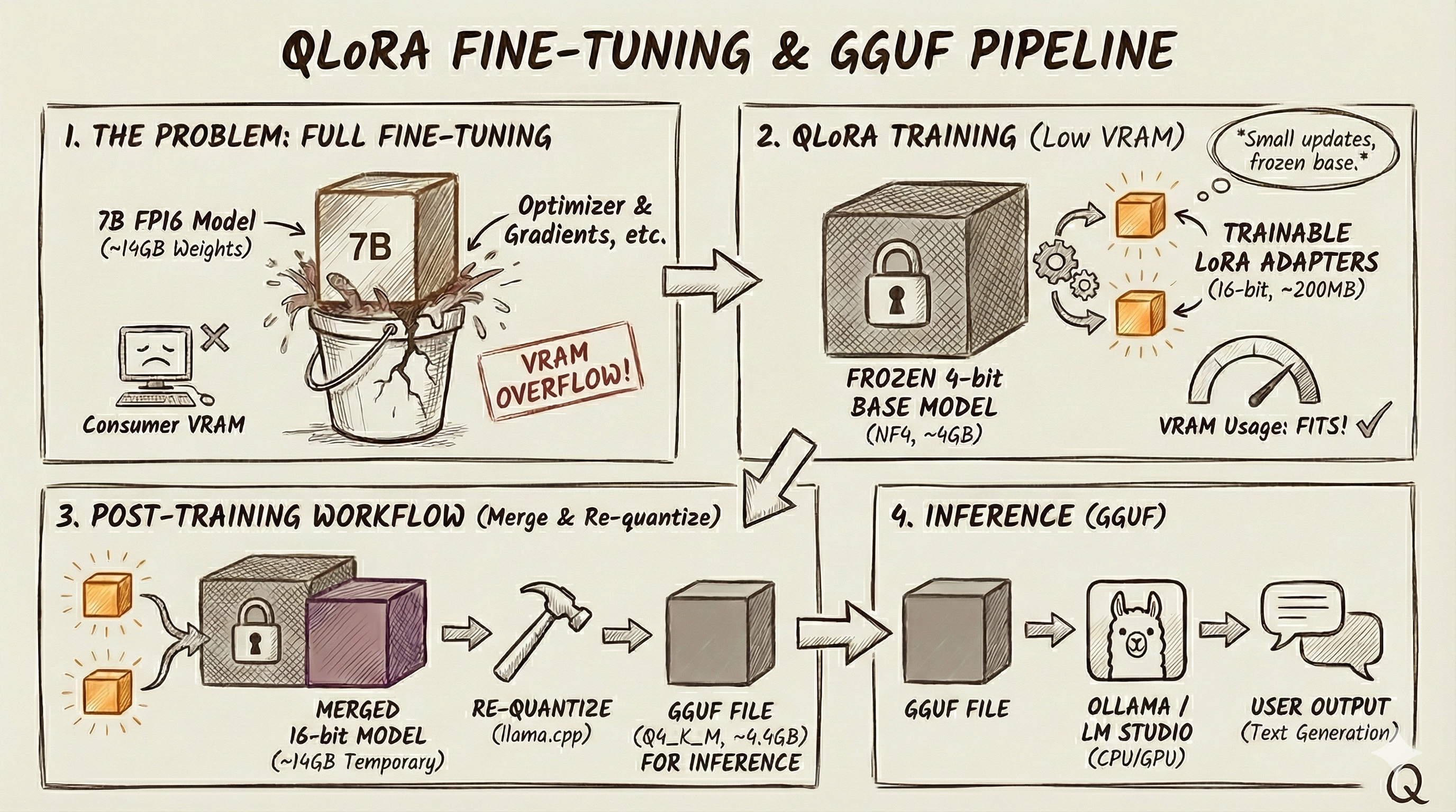
QLoRA (Quantized Low-Rank Adaptation)

Full fine-tuning a 7B model usually blows past consumer VRAM once you include optimizer state, gradients, and activations. QLoRA makes it practical by combining 4-bit quantization with LoRA adapters.

Quantization shrinks the base weights. In FP16/BF16, 7B parameters is ~14GB just for weights. In 4-bit, it’s ~3.5GB in theory and more like ~4–4.5GB in practice due to overhead. The key detail: the base model stays frozen in this compressed form during training.

LoRA avoids retraining all 7B parameters by adding small trainable “patches” to selected layers. For example, a 4096×4096 matrix has ~16.8M params. With LoRA (rank 32), you train two smaller matrices (4096×32 and 32×4096) totaling ~262K params, which combine into an update the same shape as the original. At inference, you get base model + LoRA correction.

In weight terms, a 7B 4-bit base is typically ~4–4.5GB, and LoRA adapters are usually hundreds of MB in FP16 (e.g., 80M params ≈ 160MB). Exact adapter size depends on the model, target modules, and rank—your training framework will print the real number.

ShareGPT Format

ShareGPT is a simple JSON way to store multi-turn chat data: an array of messages labeled by speaker (often “human” and “gpt”). Many fine-tuning tools (Unsloth, Axolotl, LLaMA-Factory) accept it directly, so it’s a convenient interchange format.

GGUF Format

GGUF is the llama.cpp ecosystem’s “ready to run” model container. It can bundle weights, tokenizer, and metadata in one file, supports memory-mapped loading, and is commonly what tools like Ollama and LM Studio run.

Quantization for Inference

There are two separate quantization steps:

• Training-time: load the frozen base in 4-bit (often NF4 via bitsandbytes) and train 16-bit LoRA adapters.

• Deployment-time: merge adapters into a full 16-bit model, then re-quantize to GGUF for fast local inference.

For inference I use Q4_K_M: Q4 means 4-bit, K is llama.cpp’s K-quant family, and M is the medium variant. At full 16-bit precision, a 7B model’s weights are about 14GB. Q4_K_M typically shrinks that to ~4–5GB (often ~4.4GB) while retaining good quality. Going below Q4 tends to degrade outputs more noticeably, so for security analysis where accuracy matters, Q4_K_M is usually a solid balance. This again is my understanding.

---

The Pipeline Overview

Here’s the full pipeline from raw HackerOne writeups to a model I can run locally in Ollama. The big idea is: keep the base Qwen2.5 7B model frozen and train a small LoRA adapter with QLoRA, then merge it back in and quantize to a GGUF that’s fast and small enough to deploy.

---

Implementation

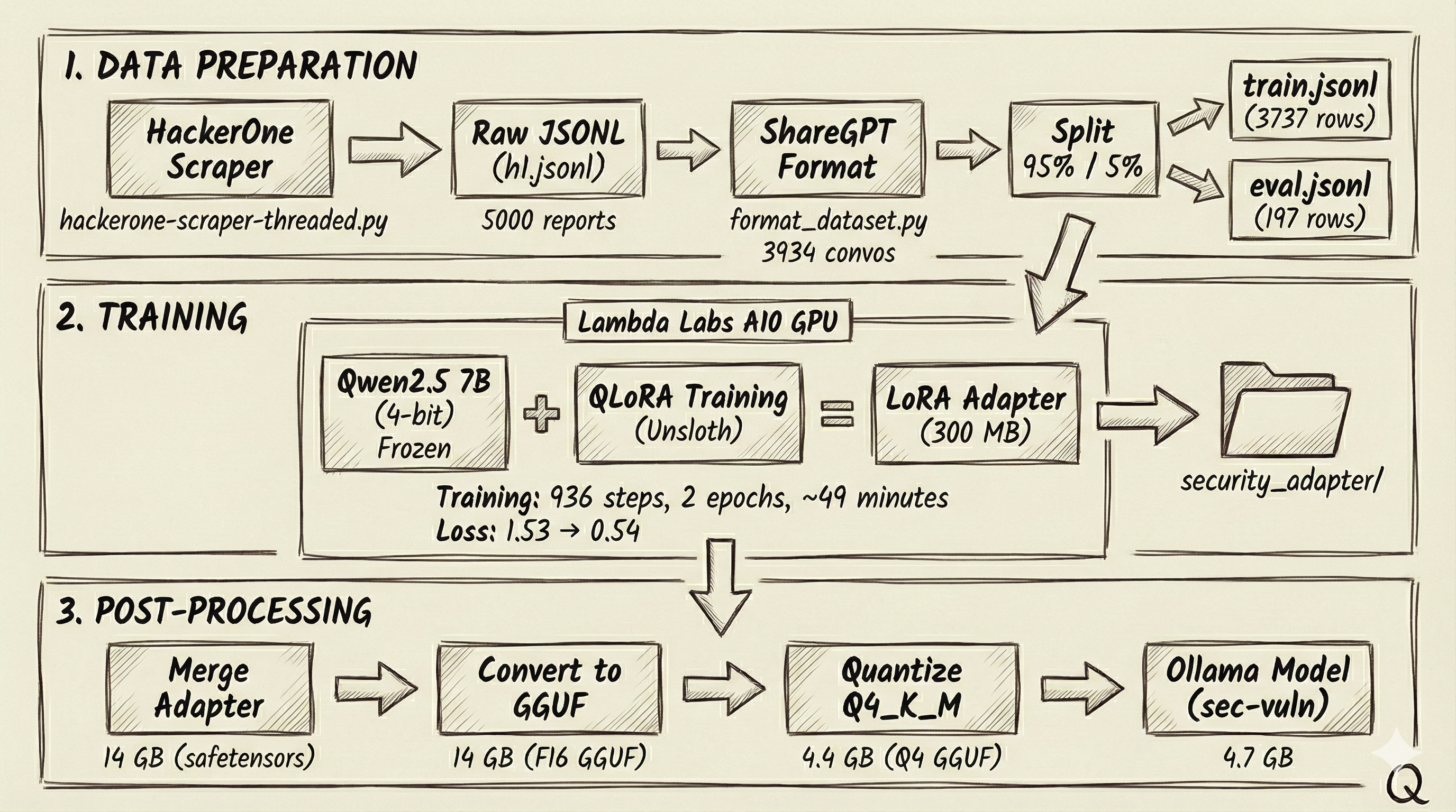
Step 1: Scraping HackerOne Reports

HackerOne’s Hacktivity page lists publicly disclosed bug bounty reports. I built a threaded scraper to collect these.

with ThreadPoolExecutor(max_workers=self.workers) as executor:
    enriched = list(executor.map(self.fetch_report, reports))

Each worker fetches report details and enforces a delay (0.5 seconds between requests) to reduce the chance of 429s/throttling. The scraper writes each enriched report as JSONL (one JSON object per line), which keeps the output streaming-friendly and easy to process later.

After ~45 minutes, I collected about 5,000 public reports (~50MB). Each record includes the vulnerability title, severity rating, program name, disclosure date, and the full report content with technical detail.

The catch (and the first lesson I missed) is that public HackerOne reports don’t reliably include the structured fields you’d expect from the GraphQL API—many come back mostly empty. When that happened, my scraper fell back to the HTML and used it as vulnerability_info. Then, because impact was often missing too, I derived it from vulnerability_info using keyword extraction, and sometimes I even reused that same meta description as the summary. The end result is the same text showing up in multiple sections of the same record—not because HackerOne duplicated it, but because I was reusing and remixing the same source text—and that matters later when you’re formatting training data and trying to build a clean train/test split.

---

Step 2: Formatting for Training

Raw vulnerability reports aren’t great training examples on their own—I needed to turn them into conversations that teach the model what kind of question it will get and what a good answer should look like.

I wrote a formatting script that converts each report into a ShareGPT-style conversation. The “human” turn includes the context (program, title, severity, URL) and asks for analysis. The “gpt” turn returns a structured write-up with clear sections like vulnerability details, impact assessment, and a short summary.

return {
    "conversations": [
        {"from": "human", "value": human_prompt},   # Analysis request
        {"from": "gpt", "value": gpt_response}       # Structured response
    ]
}

I stuck to the same markdown headers and sections each time so the model learns a predictable structure instead of dumping everything into one long blob. I also nudged the prompt away from step-by-step exploitation details. After filtering out incomplete reports (missing severity, empty content, etc.), I ended up with 3,934 valid training conversations from my initial ~5,000 scraped reports.

---

Step 3: Train/Eval Split

Before training, I needed to hold out some data for evaluation. A random split would have worked, but I used deterministic hashing for reproducibility—the same record always ends up in the same split, even if I rerun the script or add new records later.

h = hashlib.sha256(key_for(row).encode()).hexdigest()
x = int(h[:8], 16) / 0xFFFFFFFF  # Normalize to 0-1
if x < cutoff:
    # Goes to eval set

I computed the hash from a stable identifier (report ID or URL), converted it to a number between 0 and 1, and compared it against the split threshold. The nice part is that when I add new data later, the existing records stay in their original split, so I don’t accidentally contaminate the eval set.

I used a 95/5 split, which gave me 3,737 training examples and 197 held out for evaluation.

---

Step 4: Training with QLoRA

This is where the magic happens. I used Unsloth, a library that provides optimized QLoRA training. The training script does 3 things. First, it loads the base model in 4-bit quantization—this is the “Q” in QLoRA:

model, tokenizer = FastLanguageModel.from_pretrained(
    model_name="Qwen/Qwen2.5-Coder-7B-Instruct",
    max_seq_length=4096,
    load_in_4bit=True,
)

Next, it attached LoRA adapters to specific layers. I targeted the attention projections (q, k, v, o)—the core weight matrices that decide what the model pays attention to and how that attention gets written back into the output—and the feed-forward layers (gate, up, down). I used a rank of 32, which gave me enough capacity to pick up the security domain without blowing up the trainable parameter count:

model = FastLanguageModel.get_peft_model(
    model,
    r=32,
    lora_alpha=64,
    target_modules=["q_proj", "k_proj", "v_proj", "o_proj",
                    "gate_proj", "up_proj", "down_proj"],
)

Training ran with Hugging Face’s SFTTrainer. I trained for 2 epochs with a batch size of 2 and gradient accumulation of 4, for an effective batch size of 8. I used a learning rate of 2e-4, which is a common range for LoRA fine-tuning. I rented an A10 on Lambda Labs (~$0.75/hour). Training finished in about 49 minutes and took 936 steps.

During training, loss dropped from 1.53 to 0.54. One caution here: that’s training loss, not a generalization metric. With ~4,000 highly structured examples over 2 epochs, a big loss drop can also mean memorization. I didn’t track eval loss during training, so the testing section later is my primary validation. If I were doing this again, I’d monitor eval loss to catch overfitting earlier.

The headline number is that, in my configuration, I trained ~80.7 million parameters out of 7.7 billion—about 1.05% of the model. That small adapter was enough to shift output structure and pick up domain-specific vocabulary.

---

Step 5: Merging the Adapter

After training finished, I had the frozen base model and the trained LoRA adapter weights as separate pieces. For deployment, I needed to merge them into a single model.

The merge step “bakes in” the adapter by computing W' = W + A×B or each adapted layer. After the merge, the model behaves the same, but it no longer needs the PEFT/LoRA machinery at inference time.

model = model.merge_and_unload()
model.save_pretrained_merged("./security_merged_fp16", tokenizer, save_method="merged_16bit")

I saved the result in FP16 for compatibility with the GGUF conversion pipeline. The merged checkpoint came out to roughly 14GB, split across 4 safetensors files plus the tokenizer assets. This is the full-fidelity model before any inference-time quantization.

---

Step 6: Converting to GGUF

The merged model was in HuggingFace’s safetensors format—great for Python-based inference but not optimized for efficient local deployment. I converted it to GGUF, the format used by llama.cpp and Ollama.

The conversion uses llama.cpp’s convert_hf_to_gguf.py script:

python llama.cpp/convert_hf_to_gguf.py security_merged_fp16 \
  --outtype f16 --outfile security_merged.f16.gguf

The script reads the safetensors, extracts architecture metadata (context length, embedding dimensions, attention heads), and writes everything into a single 14 GB GGUF file. This intermediate F16 file preserves full precision—I’ll quantize it in the next step.

---

Step 7: Quantization

A 14 GB model is unwieldy for local use—that’s a lot of RAM to dedicate to a single application. The quantization step compresses the model to a fraction of its size.

./llama.cpp/build/bin/llama-quantize \
  security_merged.f16.gguf security_merged.Q4_K_M.gguf Q4_K_M

The quantizer processes each tensor, converting 16-bit floats to 4-bit integers with intelligent grouping. Q4_K_M uses mixed quantization across tensor types—some tensors get higher-bit treatment (like Q6_K) while others use Q4_K, depending on their sensitivity. The exact split varies by model architecture.

The result: 14 GB compressed to 4.4 GB, just 31% of the original size. Quality loss is often modest but task-dependent; I found it acceptable in my tests. The model still produced coherent, well-structured security analyses.

---

Step 8: Creating the Ollama Model

The final step wraps my quantized model in Ollama’s packaging format. A Modelfile specifies the base model, generation parameters, and system prompt:

FROM ./security_merged.Q4_K_M.gguf
PARAMETER temperature 0.2
PARAMETER num_ctx 4096
SYSTEM """You are a security vulnerability analysis assistant.
Do not provide step-by-step exploitation.
Provide root cause, impact, constraints, mitigations, and detection ideas."""

I set a low temperature (0.2) for more deterministic, focused responses—important for technical analysis where consistency matters more than creativity. Running ollama create sec-vuln -f Modelfile builds the model. Ollama creates a layered package: the GGUF weights, the system prompt, and the generation parameters each become separate layers. The final model weighs in at ~4.7 GB and is immediately available for inference via ollama run sec-vuln.

---

Testing and Validation

I created an evaluation script (eval_ollama.py) because my understanding was that training loss doesn’t tell you whether the model learned anything useful—it only tells you it got better at fitting the training distribution. I wanted a check that ran in the same setup I’d actually use (Ollama locally), so the script calls the local Ollama API and scores the tuned model on a held-out set.

For each eval record, it sends the user prompt to the model, captures the response, and compares it to the reference answer produced during dataset formatting. I tracked two buckets of metrics. The first is structure: does the output follow the expected markdown layout (## Title, ### Vulnerability Details, ### Impact, ### Summary) or does it collapse into a blob. The second is text similarity: basic token overlap metrics (precision/recall/F1 and Jaccard) to gauge how close the response is to the reference.

The script writes everything to JSONL so I can inspect results sample-by-sample. That’s how I eventually spotted the second lesson I missed: the model had learned the repetitive patterns in my training data extremely well, which can inflate similarity scores without necessarily improving real reasoning.

---

Results and Lessons Learned

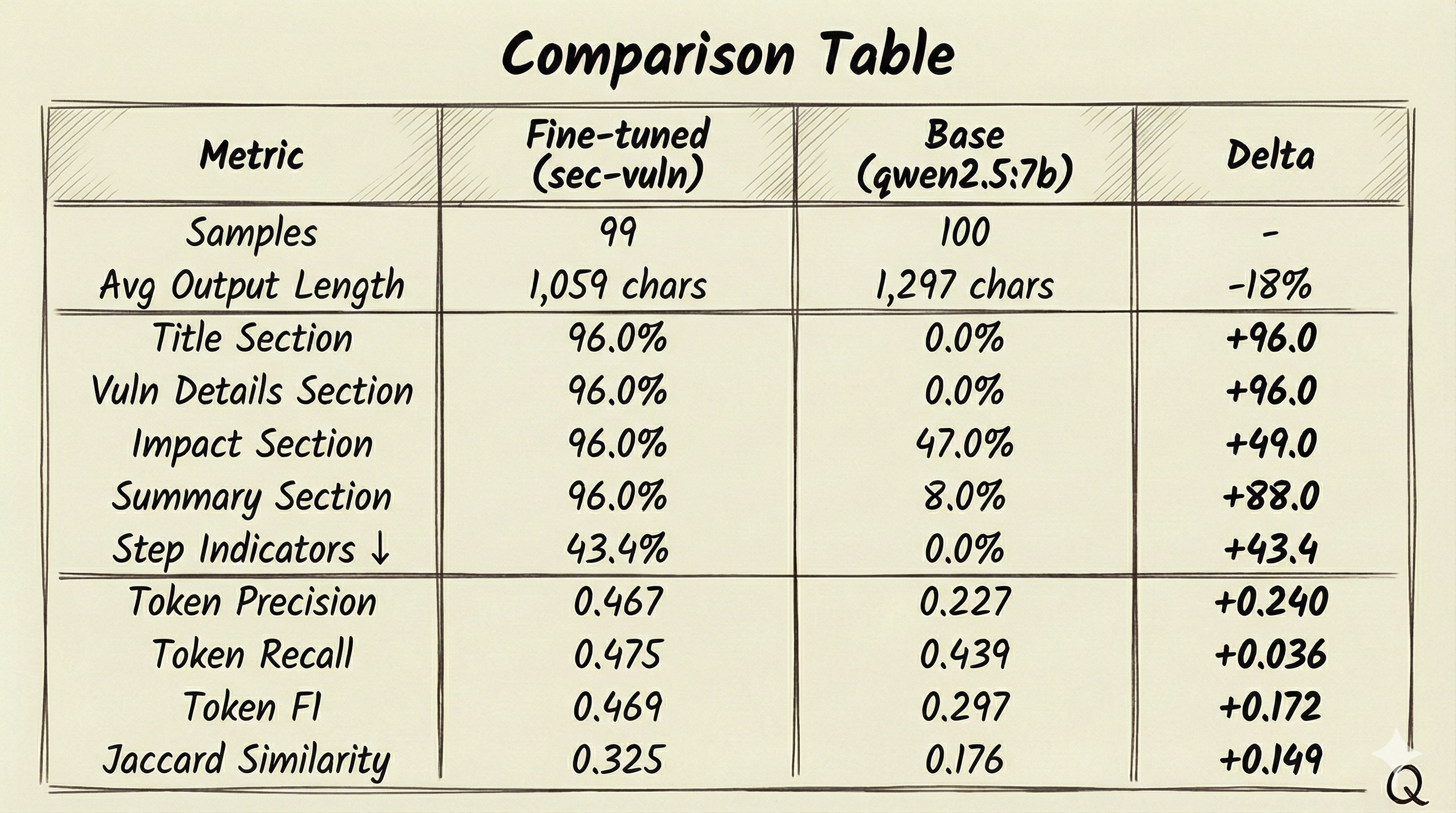
Evaluated against the 197-example held-out set using eval_ollama.py, the fine-tuned model clearly learned the output format, hitting 96% adherence to all four expected sections (vs. nearly 0% for the base model) and showing much higher token-overlap scores (F1/Jaccard), but it also picked up security-report habits, with a 43.4% “step indicator” rate—a proxy metric that flags responses containing step-by-step procedural language, which may indicate exploitation/PoC-style output (the base model stayed at 0%). The bigger issue is that these numbers look better than they really are because of the earlier data-quality problem—high adherence and overlap mostly mean the model learned to mirror repetitive training patterns (including duplicated content across sections), so the metrics confirm format compliance, not true analytical improvement.

---

Conclusion

I was pretty pumped when I first looked at the eval numbers. The tuned model was nailing the format, the overlap scores were way up, and it felt like the whole pipeline had worked exactly the way it was supposed to. Then I actually read the outputs. That’s when it clicked: the numbers looked better than they really were because of the earlier data-quality problem. High section adherence and token overlap mostly meant the model learned to mirror the repetitive training patterns—including duplicated text across sections—so the metrics were validating format compliance, not real analytical improvement. Once I traced it back through the pipeline, the facepalm moment hit, the scraper wasn’t pulling clean, independent fields. It was often falling back to the same HTML meta description, then deriving “impact” from that same text, and sometimes reusing it again for the summary. The model didn’t “discover” those repeats—it just learned exactly what I fed it.

Overall, this was a great learning journey. I really wanted to see how this all worked. My takeaway is that in fine-tuning, data quality is the whole game—if your dataset has repetition, leakage, or synthetic “structure” created by your pipeline, the model will happily learn that too, and your metrics can look great while you’re mostly measuring pattern copying.

If I got anything wrong in this write-up, please reach out and tell me—I’m learning this as I go, and I’d rather correct it than let a mistake stick.